In this notebook, I take the viewpoint of a school teacher. It is obvious that for the daily use in schools we need a more restricted set of options from EMT than for the university or for research. In the following, I try to emphasize the parts of EMT that could be helpful for such purposes blending off the advanced rest of EMT. The maximal level will be elementary calculus.
The file is in English. The author welcomes any translation, improvements or remarks.
Today, all students are capable of handling a calculator. EMT is a bit different from an ordinary calculator. To compute a complicate expression like
![]()
you need to enter it in line form.
>((1/7 + 1/8 + 2) / (1/3 + 1/2))^2 * pi
23.2671801626
Use / for dividing and ^ for powers. Carefully put brackets around sub-expressions that need to be computed first. EMT assists you by highlighting the expression that the closing bracket finishes. You will also have to enter the name "pi" for the greek letter pi.
The result of this computation is a floating point number. It is by default printed with about 12 digits accuracy.
In schools you often deal with fractions only. For this you can either print the numerical results as fractions, or use the symbolic arithmetic of EMT. We will start with the latter.
Any expression that starts with "&" is evaluated symbolically by the mighty computer algebra program "Maxima".
So let us compute the following fraction.
>& (1/7 + 1/8 + 2) / (1/3 + 1/2)
                                 381
                                 ---
                                 140
From the student viewpoint in elementary schools it may look as if symbolic computations is all that is needed. But in fact many mathematical questions do not have a symbolic answer at all. Thus there are two worlds in EMT: A fast numerical world, and a slower, but more accurate, symbolic world.
E.g., you will often have to solve equations, and often you find an exact solution. Let us try to solve
![]()
>&solve(x^2+x+1=2*x+3,x)
[x = 2, x = - 1]
We find the solutions of an equation with the "solve" command of Maxima. The answer is symbolic. There are two solutions which are presented in a list.
In the same way we can solve systems of equations. Let us try
![]()
>&solve([x^2-x-y^2=1,x+y=6],[x,y])
                                37      29
                          [[x = --, y = --]]
                                11      11
This is again a list of solutions. But in this case the list contains only one element containing the values of x and y.
Let us study the symbolic side of EMT as provided by Maxima in more detail.
First of all, Maxima has an "infinite" arithmetic which can handle very large numbers.
>&44!
2658271574788448768043625811014615890319638528000000000
This way, you can compute large results exactly. Let us compute
![]()
>& 44! / (34! * 10!)
2481256778
Of course, Maxima has a more efficient function for this (as does the numerical part of EMT).
>&binomial(44,10)
2481256778
To learn more about a specific function double click on it. E.g., try double clicking on "&binomial" in the previous command line. This opens the documentation of Maxima as provided by the authors of that program.
You will learn that the following works too.
>&binomial(x,3)
                          (x - 2) (x - 1) x
                          -----------------
                                  6
If you want to replace x with any specific value use "with".
>&binomial(x,3) with x=10
120
That way you can use a solution of an equation in another equation.
To make things easier we save the solution to a symbolic variable. That is done with "&=".
>sol &= solve(x^2+x-4=0,x)
                     - sqrt(17) - 1      sqrt(17) - 1
                [x = --------------, x = ------------]
                           2                  2
Now we use the first solution and compute its third power.
>& x^3 with sol[1]
                                          3
                            (sqrt(17) + 1)
                          - ---------------
                                   8
We probably want this expanded.
>& expand(x^3 with sol[1])
                            5 sqrt(17)   13
                          - ---------- - --
                                2        2
Using "%" we can do all that in a single line. The variable "%" refers to the last result. It should only be used within one line.
>&solve(x^2+x-4=0,x), &x^3 with %[1], &expand(%)
                     - sqrt(17) - 1      sqrt(17) - 1
                [x = --------------, x = ------------]
                           2                  2


                                          3
                          (- sqrt(17) - 1)
                          -----------------
                                  8


                            5 sqrt(17)   13
                          - ---------- - --
                                2        2
Maxima can also differentiate and integrate symbolically. Let us demonstrate that with a more complex example of Calculus. We find the area between the curves
![]()
For this, it would be nice to have these curves plotted. We will later talk about plots in more detail. But we show this simple plot right here.
We define the expressions first.
>f1 &= x^2-x, f2 &= x+1
                                 2
                                x  - x


                                x + 1
Now the simple plot command.
>plot2d(f1,-1,3); plot2d(f2,>add,color=red):
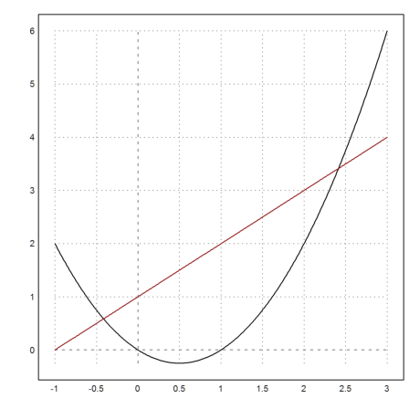
To get the area we compute the intersections.
>sol &= solve(f1=f2,x)
[x = 1 - sqrt(2), x = sqrt(2) + 1]
Now we compute the symbolic integral of the difference.
>F &= integrate(f2-f1,x)
                               3
                              x     2
                            - -- + x  + x
                              3
And finally, we evaluate it in the intersections.
>& expand( (F with sol[2]) - (F with sol[1]) )
                                  7/2
                                 2
                                 ----
                                  3
One point to criticize here is that you often get the solution and not the path leading to the solution. If you want to study the solution step by step you can do that too. Let us try to solve
![]()
We first store the two equations in two symbolic variables.
>eq1 &= (x^2+y^2+x=6), eq2 &= (x+y=3)
                            2    2
                           y  + x  + x = 6


                              y + x = 3
Next we eliminate x from the first equation.
>&solve(eq2,x), &eq1 with %, res &= expand(%)
                             [x = 3 - y]


                       2              2
                      y  - y + (3 - y)  + 3 = 6


                            2
                         2 y  - 7 y + 12 = 6
Now we solve this quadratic equation by quadratic extension. The trick is that any arithmetic operation is applied to both sides of an equation, just as it should be.
>& expand(res/2), & %-6+(7/4)^2, & factor(%), & %*16
                            2   7 y
                           y  - --- + 6 = 3
                                 2


                           2   7 y   49   1
                          y  - --- + -- = --
                                2    16   16


                                    2
                           (4 y - 7)    1
                           ---------- = --
                               16       16


                                     2
                            (4 y - 7)  = 1
We arrive at a form that allows us to compute the solutions y=2 and y=3/2 in our head. Indeed
>&solve([eq1,eq2],[x,y])
                                         3      3
                   [[x = 1, y = 2], [x = -, y = -]]
                                         2      2
The students leaves the realm of fractions and square roots as soon as trigonometric functions, exponentials or logarithms are involved. Then they need a pocket calculator to get a result.
The output of a numerical calculator are "floating point numbers". Those have a fixed number of correct digits (about 16). EMT prints only 12 digits by default.
For an example, we compute the height of a tower in 100m distance. The top of the tower was measured 10.5 degrees above the horizon.
>100*tan(10.5°)
18.5339044932
Use F7 to get the degree symbol if you do not have a key for it.
Of course, not all printed digits make sense. Depending on the accuracy of the measurements, the result can be different.
>100.4*tan(10.4°)
18.4268481966
EMT can print results in many different formats. E.g., the length of the output can be changed for a single value quite easily.
>shortest 1/3, short 1/3, long 1/3, longest 1/3
    0.333
0.33333
0.333333333333
     0.3333333333333333
Or you can set a specific format for all output.
>format(10,2); exp(5.6)
270.43
In any case, "defformat" brings you back to the default format. Of course, restarting EMT does the same.
>defformat; exp(5.6)
270.426407426
Students meet floating point numbers also in natural sciences. EMT can convert units to the international system (meter, seconds, kilograms).
>115yards, 2.5miles, 3ft, 1lightyear
105.156
4023.36
0.9144
9.46073047258e+015
The last result means about 9.5 times 10^15 meters.
EMT can also convert between units.
>3d->min // days to minutes
4320
It is possible to append the unit as a string. Note, that fractions of units are also possible.
>500ft/min -> " m/sec"
2.54 m/sec
Also, the unit % stands for 1/100 simply.
>4567.89*19%
867.8991
For most real world problems there is no symbolic solution at all. E.g. the expression
![]()
has a unique solution. But we can find it only with numerical methods. The function "solve" is the numerical counterpart of "&solve" from Maxima. It finds the solution with the Secant method. But it needs a starting guess.
>xsol = solve("cos(x)-x",1)
0.739085133215
Let us plot the two functions and the solution. Above, we have stored the solution in the numerical variable "xsol" with "=".
>plot2d("cos(x)",0,pi); plot2d("x",>add); plot2d(xsol,xsol,>points,>add):

As you see, to be able to plot a solution is a nice check for its correctness. Of course, we can also check the values directly.
>xsol, cos(xsol)
0.739085133215
0.739085133215
In natural science and in mathematics we often meet data sets in vectors.
To learn about vectors, we generate a random vector of dice throws.
>v = intrandom(10,6)
[4, 2, 6, 2, 4, 2, 3, 2, 2, 6]
EMT has a lot of functions for vectors. E.g. we can compute the sum or the product of the elements of a vector.
>sum(v), prod(v)
33
55296
Using the colon operator a:b, we generate a vector of numbers from a to b.
>1:10, prod(%), 10!
[1,  2,  3,  4,  5,  6,  7,  8,  9,  10]
3628800
3628800
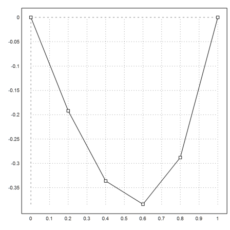
Vectors are also useful for tables of functions.
>t=0:0.2:1, s=t^3-t
[0,  0.2,  0.4,  0.6,  0.8,  1]
[0,  -0.192,  -0.336,  -0.384,  -0.288,  0]
The trick here is that t^3-t is applied to every element of t. This is called "vectorization" of operators and functions.
We can now plot the values as points or as lines with points.
>plot2d(t,s,>addpoints):
To find the extremal values, we can use min(t) and max(t). Or we can find the indices of these extremal values together with the values.
>min(s), max(s), extrema(s)
-0.384
0
[-0.384,  4,  0,  1]
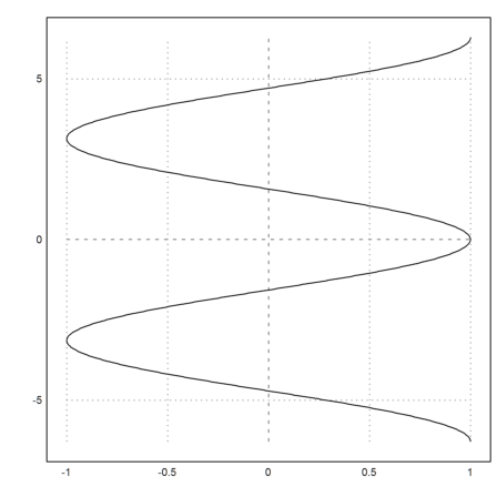
Plotting data vectors is an alternative to the plot of functions or expressions. The advantage is that you get a lot more control now. E.g., let us plot the relation
![]()
To generate a vector of values for y we use linspace() now.
>y=linspace(-2*pi,2*pi,1000); x=cos(y); plot2d(x,y):
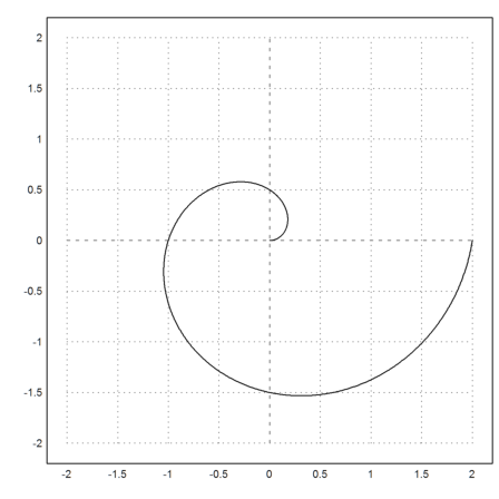
Then, of course, we can also plot curves.
![]()
with plot(x,y) where x is a vector of x-values, and y is a vector of y-values.
>t=linspace(0,2*pi,1000); plot2d(t/pi*cos(t),t/pi*sin(t),r=2):
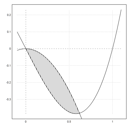
Since curves can be filled we can now fill any area that is bounded by a curve.
The following is a bit tricky. First of all, we use a nulti-line. Such lines are concatenated with "...". Press Ctrl-Return to extend the current line to a multi-line, or to split a line into two lines.
We plot two functions, and compute their intersection b=0.61. Then we let x walk from 0 to b and back, with the values stored in a vector (x|xi appends two vectors).
>plot2d("x^3-x",-0.1,1.1); plot2d("-x^2",>add);  ...
 b=solve("x^3-x+x^2",0.5); x=linspace(0,b,200); xi=flipx(x); ...
 plot2d(x|xi,x^3-x|-xi^2,>filled,style="|",fillcolor=1,>add):
There are also other styles for plots of data. E.g. let us demonstrate the Riemann sum below the function y=x^2.
>plot2d("x^2",0,1); plot2d(0:0.1:1,(0:0.1:0.9)^2,>bar,>add):
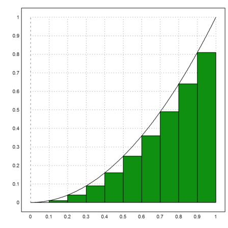
We can easily compute the sum of the green bars.
>t=0:0.1:0.9; sum(t^2)*0.1
0.285
Another use of vectors is the study of limits and sums. The following computes
![]()
>sum(1/(1:1000000)^2), pi^2/6
1.64493306685
1.64493406685
Matrices may be studied in schools. The matrix algebra is usually not a topic, but representing a linear system of equations in matrix form may be. Matrices can also be used for tables.
To be able to print our matrices without line breaks, we set a short fractional format.
>fracformat(8); A = [1,2,3;4,5,6;7,8,9]
      1       2       3
      4       5       6
      7       8       9
Operators vectorize to matrices too.
>1/(A*A)
      1     1/4     1/9
   1/16    1/25    1/36
   1/49    1/64    1/81
The matrix product of Linear Algebra is denoted by a dot.
>A.A
     30      36      42
     66      81      96
    102     126     150
The lines of A are A[k] etc., and the columns A[,k]. Let us compute the determinant of A using the Gauss algorithm.
>A[2]=A[2]-4*A[1]
      1       2       3
      0      -3      -6
      7       8       9
>A[3]=A[3]-7*A[1]
      1       2       3
      0      -3      -6
      0      -6     -12
>A[3]=A[3]-2*A[2]
      1       2       3
      0      -3      -6
      0       0       0
The determinant is 0.
If you want to check a Gauss computation you can use the function pivotize(), which does many steps in one.
>A=[1,2,3;4,5,6;7,8,10]; b=[1;1;1]; M=A|b
      1       2       3       1
      4       5       6       1
      7       8      10       1
>pivotize(M,1,1)
      1       2       3       1
      0      -3      -6      -3
      0      -6     -11      -6
>pivotize(M,2,2)
      1       0      -1      -1
      0       1       2       1
      0       0       1       0
>pivotize(M,3,3)
      1       0       0      -1
      0       1       0       1
      0       0       1       0
We read the solution of Ax=b from this as x=-1, y=1, z=0.
Of course, we can also get the solution with a command.
>A\b
     -1
      1
      0
To use matrices for tables, let us reset to the default format, and compute a table of sine and cosine values. Note that angles are in radians by default.
>defformat; w=0°:45°:360°; w=w'; deg(w)
            0
           45
           90
          135
          180
          225
          270
          315
          360
Now we append columns to a matrix.
>M = deg(w)|w|cos(w)|sin(w)
            0             0             1             0
           45      0.785398      0.707107      0.707107
           90        1.5708             0             1
          135       2.35619     -0.707107      0.707107
          180       3.14159            -1             0
          225       3.92699     -0.707107     -0.707107
          270       4.71239             0            -1
          315       5.49779      0.707107     -0.707107
          360       6.28319             1             0
The statistical package contains a command to read and write matrices. Let us abuse that for our matrix.
>writetable(w|sin(w)|cos(w),labc=["rad","sin","cos"],labr=deg(w))
                 rad       sin       cos
         0         0         0         1
        45      0.79      0.71      0.71
        90      1.57         1         0
       135      2.36      0.71     -0.71
       180      3.14         0        -1
       225      3.93     -0.71     -0.71
       270      4.71        -1         0
       315       5.5     -0.71      0.71
       360      6.28         0         1
Maxima has symbolic matrices. We restrict ourselves to a short demonstration.
>A &= [a,1,1;1,a,1;1,1,a]
                             [ a  1  1 ]
                             [         ]
                             [ 1  a  1 ]
                             [         ]
                             [ 1  1  a ]
>&det(A), &factor(%)
                             2
                         a (a  - 1) - 2 a + 2


                                  2
                           (a - 1)  (a + 2)
>&invert(A) with a=0
                          [   1   1    1  ]
                          [ - -   -    -  ]
                          [   2   2    2  ]
                          [               ]
                          [  1     1   1  ]
                          [  -   - -   -  ]
                          [  2     2   2  ]
                          [               ]
                          [  1    1     1 ]
                          [  -    -   - - ]
                          [  2    2     2 ]
Probability theory and statics are nice topics for the school since they have immediate real world applications. EMT has a lot of statistical functions and methods. Let us concentrate on two basic distributions: the binomial distribution and the Gaussian distribution.
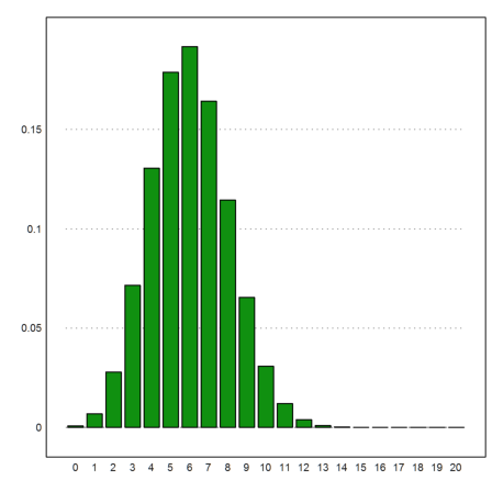
First, let us plot the binomial distribution.
![]()
Again, we use the matrix language of EMT to compute the vector of values for a fixed n. The functions columnsplot() is one of the statistical plots of EMT. It needs a vector of labels for the x-axis.
>n=20; k=0:n; p=0.3; columnsplot(bin(n,k)*p^k*(1-p)^(n-k),lab=k):
Let us do some Monte-Carlo simulations.
The function intrandom(N,n) generates N integer values from 1 to n, each with equal probability.
>intrandom(10,6)
[2, 5, 2, 3, 2, 6, 2, 3, 1, 4]
If we do that 6000 times, we should get each number about 1000 times.
>v=intrandom(6000,6); getmultiplicities(1:6,v)
[978, 1002, 981, 988, 1008, 1043]
Besides using "getmultiplicities" we can also use the matrix language to count for the number 6 in the following way. Note that "==" compares two values for equality and yields 1=true or 0=false. It works for each element of a vector.
>[1,2,3,6,5,4,6], %==6, sum(%)
[1,  2,  3,  6,  5,  4,  6]
[0,  0,  0,  1,  0,  0,  1]
2
It is possible to write loops to achieve the same result. For users with elementary programming languages this looks as the easiest way. It is far slower, however.
>v=[1,2,3,6,5,4,6]; ...
 k=0;  ...
 for i=1 to length(v); ...
   if v[i]==6 then k=k+1; endif; ...
 end; ...
 k
2
EMT has the Gaussian distribution and its inverse, of course.
Let us compute the probability that 1020 times the number 6 is found in 6000 random integers selected from 1 to 6. The theory tells us that the distribution of the number of 6 is approximately Gaussian with
![]()
with n=6000, p=1/6.
>n=6000; p=1/6; mu=n*p; sigma=sqrt(n*p*(1-p)); 1-normaldis(1020,mu,sigma)
0.244211158311
Instead of simulating this with a loop we use a matrix of 1000 lines with 6000 random number in each line, and let the matrix language of EMT do its services.
>N=1000; n=6000; v=sum(intrandom(N,n,6)==6)';
Now, v is vector of counts of 6 in each line. The "plot2d" function can plot the distribution of these counts. We add the density function of the normal distribution to the distribution of the values.
>plot2d(v,>distribution); plot2d("qnormal(x,mu,sigma)",>add,color=red):
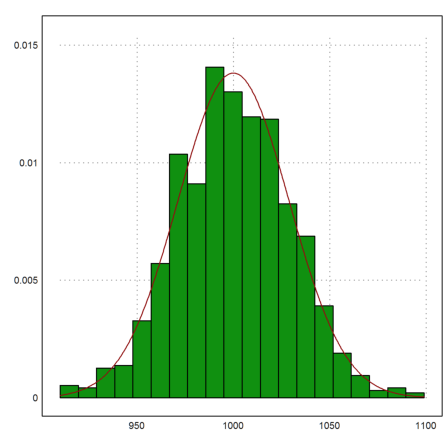
We should get approximately 240 times more than 1020.
>sum(v>=1020)/N
0.259
We could ask the inverse question too. Determine a count K such that more than K hits are not expected with probability less than 5%.
>invnormaldis(0.95,mu,sigma)
1047.48283421
Thus we can compute an interval where the count is "with 90% probability".
>invnormaldis([0.05,0.95],mu,sigma)
[952.517, 1047.48]
We can also randomly shuffle a vector. E.g., we can select randomly 6 out of 49 with one command. The trick is to shuffle the numbers 1 to 49, and then take the first 6 elements of the shuffled values.
>sort(shuffle(1:49)[1:6])
[5, 15, 16, 18, 27, 39]
It is interesting to ask how many numbers stay at their places when a vector from 1 to n is shuffled. Let us simulate that 1000 times and get the mean number of fixed points. The expected value is known to be 1.
>k=0; N=1000; loop 1 to N; k=k+sum(shuffle(1:49)==1:49); end; k/N
0.934
As you see, EMT can well be used for Monte-Carlo simulations. If the matrix language does not work for a particular problem and the programming language of EMT is too slow, Python or C can also be used.
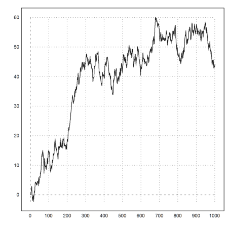
For a final example, we generate a random walk with 0-1-normal distributed steps.
>plot2d(0|cumsum(normal(1000))):
Teachers often need plots that can be printed. EMT can export vector graphics too. But for most purposes, images are sufficient. We face two main problems.
Assume, we want to print the sine and cosine functions on a page with 10cm width and a font of 8pt height in a 2:1 ratio.
>aspect(2); setfont(8pt,10cm); plot2d(["sin(x)","cos(x)"],0,2pi):
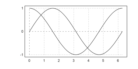
To print such a plot I recommend to save it without anti-aliasing to a PNG. Simply select "For Print". You get a 2000x1000 pixel file which is good enough for a print width of 30cm. You can include a PNG in PDF-Latex or in any Word document.
To reset to the default values use "reset".
>reset;